hexagonal grid or no hexagonal grid

Every now and then I find documents about hexagonal grids or hexagonal image processing where the authors appear to have a different understanding of the term 'hexagonal' than I have. Today I found such a document again, and this time I want to share my opinion...

Rotated square Grid
A simple internet search lead me to a paper with the title 'Demosaicking of Hexagonally-Structured Bayer Color Filter Array'. Seems like someone shares my interests in hexagonal grids and color filter arrays. And somehow the author figured out a way to apply something like a Bayer pattern to a hexagonal grid. That is indeed interesting! So I started reading the abstract and there it was:

"[...] The hexagonal CFA can be considered to be a 45-degree rotational version of the Bayer pattern [...]"

No, a hexagonal CFA cannot be considered as a rotated version of the Bayer pattern! Rotating a sqare grid (which is the basis for the Bayer pattern) results in a rotated square grid, not in a hexagonal grid! 

Let me outline what I believe a hexagonal grid is: A (regular) hexagonal grid is one in which every element has six neighbors with the same distance. Drawing lines from the center of one of these neighbors to the next results in a regular hexagon. A hexagon is a shape with six sides and six corners. In the special case of a regular hexagon (which I assume is the most practical one) all sides have the same length and all corners have the same angle. The single elements don´t have to be hexagons necessarily, these may also be e.g. circles.
Well, that sounds a little more scientific than I wanted it to. To make it a little simpler you could also say in a hexagonal grid it should be possible to identify hexagons.

Coming back to the paper I have to say that I can´t read the content as it is Korean. However, the authors also provide an image of what they call a hexagonal color filter array.

Okay... in the abstract they say, they rotated the Bayer pattern to get a hexagonal pattern. This is not what I see here (Again, I have to emphasize that I can´t read the paper. I am just assuming that the figure demonstrates the process described in the abstract). What I see is that they rotated the grid and then changed the distance between the elements. I have no idea why they would do that as it makes the grids incomparable. But that´s another topic. The main point is: the figure to the right does not show a hexagonal grid. What is shows is Fuji´s SuperCCD design.

Fuji SuperCCD

Fuji´s SuperCCD sensors have often been described with 'hexagonal' or 'honeycomb'. But that´s not correct. SuperCCD is just a rotated square grid. Well, to make it look more interesting, the marketing guys have chopped off the corners of the squares to produce octagons (!), but these were still placed on a square grid.

The figure above illustrates the layout of the SuperCCD sensors. By rotating the grid Fuji´s scientists achieved to get a grid on which the green pixels were placed on a horizontally aligned square grid. Compared to that, the green pixels are placed on a rotated grid in the conventional Bayer pattern. The advantage of such a layout should be that horizontal and vertical lines (which are assumed to be dominant in natural images) may be reproduced better. However, my experience is that the exact opposite is the case. The missing green pixels are much easier to interpolate horizontally or vertically than diagonal. But there may be algorithms which can handle that.

The pixels´ octagonal shape is a pure marketing gag in my opinion. What would it help to reduce the light sensitive area? Fuji has always claimed that the SuperCCD sensors are more light sensitive than their competitors. Well, that is possible, but the reason for that is for sure not the octagonal shape of the pixels. Maybe it is because they found a way to decrease the distance between the pixels (which is not represented in the figure above) or they simply have better material than the others, but there´s no logical explanation why chopping off the pixel´s edges would increase sensitivity.

I think I am slightly off-topic... 

Conclusion

What I´m trying to say is that neither SuperCCD, nor the layout from the paper on top is hexagonal. When I found articles on the internet ten years ago, describing SuperCCD as 'hexagonal', I was wondering, but I didn´t care too much. But when I find scientific work that was published only recently, in which those things are mixed up, then I am a little worried. I am not saying that the algorithm described in this paper is bad. I´m just saying that people who invent image processing algorithms should know the difference between a square and a hexagon. Especially in scientific work this differentiation should be taken serious. I believe that hexagonal image sampling and processing has great potential which is yet unused. I wish more people investigated in (real) hexagonal image science and publish their work. And those trying to find this work should not have to examine if a certain paper really deals with hexagonal image processing or has just a wrong title.

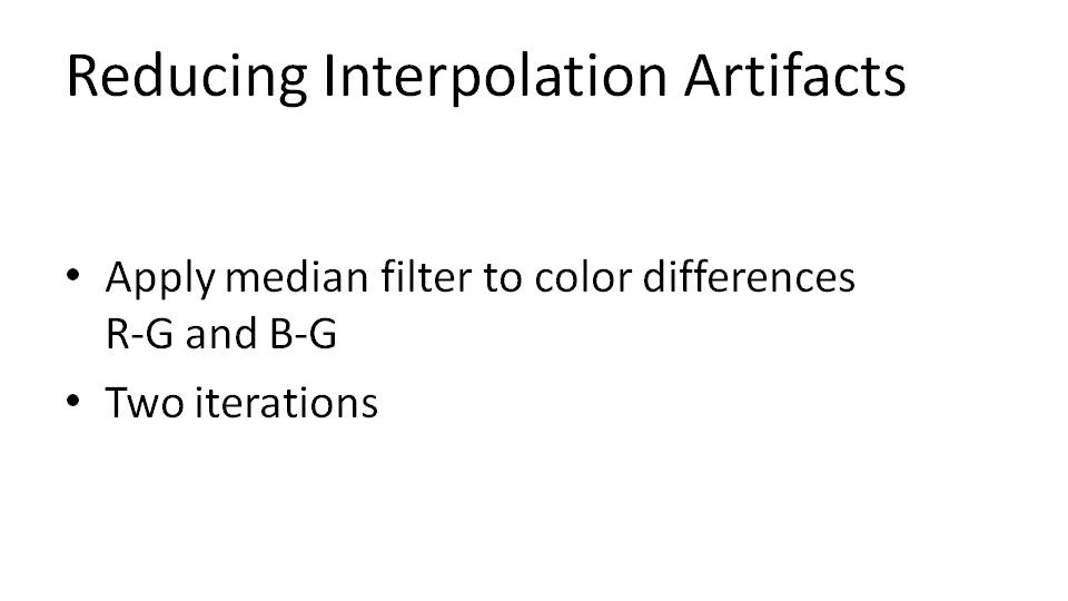
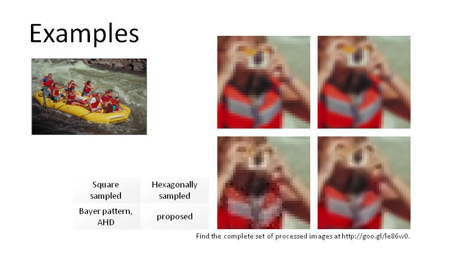
"A Novel Color Filter Array and Demosaicking Algorithm for Hexagonal Grids" slides

I have already mentioned my paper in earlier posts. Today I want to share the slides that I used when I presented the paper in China at ICGIP 2014.

Displaying hexagonal sampled images

In my earlier posts I added some images enlarged so much that the hexagonal nature of their sampling is visible. You may have wondered how I created these images so that they can be shown in your browser, knowing that there is no image file format that supports hexagonal images. In fact, I had to figure out a way to convert these hexagonal sampled images into square sampled images - but not in a way as you would do it if you want to convert an image from a hexagonal sensor. Because in this case you would want to suppress the visibility of the sampling grid. In my case I wanted to do the exact opposite - I wanted to emphasize the sampling grid.
Well, I guess I could have done it Matlab, as kindof the opposite of the hexagonal resampling operation that I explained in an earlier post. This would have been sufficient for online publishing. But when I first started doing this in 2010 I wanted to have a vector graphic which I could insert into my diploma thesis, so that the images would be rendered in the best possible quality, independent of the actual resolution of the print. Therefor I decided to store the hexagonal images as svg files using some Matlab code. I could then open these svg files in Inkscape, a free vector graphics tool, and save it in any other file format, e.g. pdf for printing (and also viewing on the moditor while still maintaining the nature of a vector graphic) or as png with any desired resolution.
So, to make it short, this is how it works:

1. export the hexagonal sampled image as svg file (using some matlab code)
2. open the svg file in Inkscape
3. export a png file

You can find the Matlab code at the end of the post. Please note that it is not perfect (I didn´t plan to make it public first and I was too lazy to fix all issues later). For example, the area that is used for the hexagonal grid is calculated incorrect, so you may need to fix the page size in your svg editor.

One thing that you should consider is that the svg files are huge as every pixel requires about 100 bytes (compared to three bytes in a bitmap graphics file).

Using Inkscape I found that the export as png works best with 2dpi. This will produce images in which each hexagon is roughly 40 pixels high. You can then scale this image to any smaller size you like. When scaling, make sure not to use bicubic or lanczos interpolation as these will introduce artifacts at the edges of the hexagons. better use bilinear (triangle) interpolation.

function [  ] = HexImWriteSVG( HexImage, Filename )

% writes a hexagonally sampled image to SVG

%check datatype of input image and convert to uint8

if isa(HexImage,'uint8')

    %do nothing

elseif isa(HexImage,'uint16')

    HexImage=uint8(HexImage/2^8);

elseif isa(HexImage,'double')   

    if max(max(max(HexImage)))>1

        fprintf('HexImWriteSVG Error: unsupported data type.\n'); return

    else

        HexImage=uint8(HexImage*2^8);

    end

else

    fprintf('HexImWriteSVG Error: unsupported data type.\n'); return

end

        

HexImageSize=size(HexImage);

HexImageWidth=HexImageSize(2);

HexImageHeight=HexImageSize(1);

%open file for writing

fId = fopen(Filename,'w+');

if (fId < 3)

    fprintf('HexImWriteSVG Error: Failure to open the output file.\n');

    return

end

    

%write SVG

fwrite(fId,['<svg width="' num2str((HexImageWidth+2)*1500) '"  height="' num2str((HexImageHeight+2)*1700) '"><g id="layer1">']);

for y=1:HexImageHeight

    for x=1:HexImageWidth

        fwrite(fId,['<path d="M'...

            num2str((x * 1.5)*980) ','...

            num2str((0.866 + y*1.732 - mod(x,2)*0.866)*980) ' l -500,866 l 500,866 l 1000,0 l 500,-866 l -500,-866 z" style="fill:#'...

            dec2hex(HexImage(y,x,1),2)...

            dec2hex(HexImage(y,x,2),2)...

            dec2hex(HexImage(y,x,3),2) ';" />']);

    end

end

fwrite(fId,'</g></svg>');

fclose(fId);

Conversion from the hexagonal grid to the rectangular grid (part 2)

While I only provided a brief introduction about how the algorithm works in the previous post, I will now try to explain in detail how it converts a hexagonal image into a square image. For easier understanding I will also present sample images for each step.

The hexagonal image

The starting point is a hexagonally sampled image. Note that the orientation of the hexagonal grid is selected so that every pixel has a corner left and right and a flat edge on the top and at the bottom. This means that every other column is shifted by 0.5 * pixel height. Of course the algorithm can also be programmed to accept hexagonal images with a 90° rotated grid, however, I always refer to this orientation.

So, here´s the hexagonally sampled image which I will use for the demonstration:

The image is actually stored in a normal two-dimensional array. Displaying this array like a normal image using Matlab´s imshow() command looks like this:

The shift of every other column is easily recognizeable in horizontal edges. By comparing both images you can also see that the aspect ratio is different. While the upper image uses hexagonally shaped pixels and therefore has a correct aspect ratio, the lower image uses square pixels to represent the hexagonal pixels which were used in image sampling. The hexagonal grid actually has a pixel aspect ratio of 1:1.1547 while the square grid has 1:1. This means that the second image appears about 15% wider than it should.

Expand to rectangular grid

The first thing that needs to be done is to fix the pixel shift. For this, the algorithm introduces new pixels in the image to produce a checkerboard pattern.

This will - obviously - again result in an incorrect pixel aspect ratio of 2:1.1547 or 1:0.5774.

Interpolation

The next step is the most tricky one: the new black pixels need to be filled with color. Obviously, we will use the surrounding pixels to interpolate the missing values.

 

The figure above shows the center positions of the pixels which are available for the interpolation as well as the center position of the pixel for which we want to calculate the color values. As it is exactly on the border between the above and below pixel, one could assume that using only these two pixels for the interpolation would be a good approach. However, the result is rather unsatisfying:

Applying a vertical linear interpolation results in a image where horizontal edges show strong artifacts. Another approach could be to use a weighted average of horizontal interpolation and vertical interpolation. The weights should represent the distances between the pixels on the horizontal and vertical axes, respectively. Therefore the vertically interpolated value needs to be weighted 1.7321 times stronger than the horizontally interpolated value.

In fact, the image looks even worse than the vertical-only interpolated image. Here, not only horizontal edges, but also vertical edges show strong artifacts. 

The solution is adaptive interpolation. The algorithm has to find whether horizontal interpolation or vertical interpolation leads to the best result. Therefore, it needs to analyze the image. It does this by analyzing each pixel´s neighbourhood in horizontal and vertical direction. The differences of a pixel´s values and those of its neighbours in each direction are stored in a map as displayed below.

Here you can see red areas where there are vertical edges and blue areas where there are horizontal edges. This map will then be blurred and finally used as a basis to decide if a pixel´s values shall be taken from the horizontally interpolated image or from the vertically interpolated image.

The combined image will then look like this:

Fixing the aspect ratio

Finally, the aspect ratio needs to be fixed. There are two options to do this: either stretch the image horizontally or squeeze it vertically. The results are as follows:

The horizontally stretched image measures 154*237 pixels (compared to the hexagonally captured 89*118 pixels). The total pixel count is more than three times higher than the pixel count of the captured hexagonal image.

The vertically squeezed image measures 89*136 pixels an has roughly 15% more pixels than the original hexagonal image. It appears less processed than the stretched image, but when having a closer look you will find that quite some detail is missing compared to the stretched image.

Code

hex_to_rect.m
This file contains the Matlab code to do the conversion. Feel free to use it and improve it. I will be happy about your feedback.

Conversion from the hexagonal grid to the rectangular grid (part 1)

In an earlier post I proposed a method to create hexagonally sampled images in order to overcome the problem of missing hexagonal image sensors. In this article I want to show you how to convert a hexagonal image into a rectangular image.

The algorithm quickly explained

First of all the algorithm expands the hexagonal image in vertical direction by introducing black pixels between the existing ones. The goal is to have a grid without 0.5-pixel shifts, as we have it in the hexagonal grid. After stretching the image, we have a checkerboard pattern.
The next step is to interpolate the values at the new pixel positions. There are various ways to do this. The easiest would be to use bilinear interpolation. However, I found that with a non-adaptive interpolation you will still be able to recognize the hexagonal pattern in the final image. This is why I designed the algorithm to first create two candidate images, one horizontally interpolated, the other vertically interpolated. After that the algorithm decides at every pixel position from which of the candidate images to take the color values.
After that you end up with a fully interpolated image with a weird pixel aspect ratio. You can now stretch or squeeze the image to achieve a pixel aspect ratio of 1:1. Horizontal stretching will make the resulting image much bigger than necessary, vertical squeezing may result in loss of information (even though the pixel count will still be higher than that of the original hexagonal image).

Sample images

Below there are some processed images. The left image is the hexagonally sampled image. The middle image has a rectangular grid, it is derived from the left image. The image to the right is a square sampled image for comparison.

Pixel count

It is quite obvious that the middle column (rectangular grid, derived from hexagonal grid) has much more pixels than the right column (square sampled images). This is due to the nature of the conversion. Of course, the rectangular image can be resized to have the same resolution as the square sampled image. However, this might result in loss of information. So, in order to keep as much information as possible in the images, I decided to leave them at the higher resolution.

Skewed edges

The higher resolution actually doesn´t bring much visible detail. Instead it makes the image look smoother. However, in some of the test images you may see that skewed edges look better in the middle column than in the right column. It is not so obvious in the posted examples, but hexagonal sampling has advantages in rendering skewed lines and also with high vertical frequencies (provided that you use the same orientation of the grid as I do). This is because on the hexagonal grid every other column is shifted by 0.5 pixels. This allows to introduce sub-pixel interpolation and achieve some gain in vertical resolution. However, the effect is only visible in few situations.

Artifacts

The conversion algorithm decides at every sub-pixel location whether to interpolate horizontally or vertically, depending on the surroundings. In some situations, especially when there´s a lot of fine detail, it happes that the algorithm makes a wrong decision which leads to visible artifacts (an example for that is the tree in the 'lake' image). However, all the images have been sampled without anti-aliasing filtering. In real world applications the situations in which artifacts are introduced would be much less. But anyway, there is room for improvement.

Code

hex_to_rect.m
This file contains the Matlab code to do the conversion. Feel free to use it and improve it. I will be happy about your feedback.

In part 2 I explain in more detail how the algorithm works.

hexagonal resampling

Introduction
Hexagonal image processing is a somewhat exotic part of imaging science. Digital images are typically considered as a number of pixels arranged in a square lattice. This is actually not predefined by nature, it is just the easiest way to describe two-dimensional data - which images are. Another way of representing such two-dimensional data is in the form of hexagonal lattices. There are actually scientists who have shown that hexagonal sampling is more efficient than square sampling. There are also scientists who investigated the performance of certain image processing algorithms on square and hexagonal lattices to prove that hexagonal sampling also enhances computational efficiency. What I found in most of these papers is that the authors typically don´t spend much time for the gathering the hexagonally sampled images. The biggest problem in hexagonal image processing currently is that there is no way to capture images on a hexagonal lattice, simply because there exists no such image sensor. So the only way to process hexagonal images is to create them artificially. In this article I will propose a method to create hexagonally sampled images.

Method

There are rather simple ways to create hexagonally sampled images from square sampled images. You could for example stretch the square sampled image using a simple interpolation method and then ignore every other pixel so that you end up with a virtual hexagonal grid. Other similar methods are used in the existing literature. What is common to all of them is that they try to convert the square sampled image into a hexagonally sampled image with approximately the same pixel count. This is actually a process which will always introduce loss of information and it is a very poor approximation of hexagonal sampling. What these approaches ignore is the fact that hexagonal sampling not only requires a hexagonal lattice, it also requires hexagonal shaped pixels. You can´t simply take a square pixel, put it into a hexagonal grid and call it a hexagonal pixel. So, what I propose is a resampling algorithm which imitates 'real' hexagonal sampling. Real image sampling means that there is a natural scene which reflects light into a camera´s lens. The lens may introduce some distortion which limits the spatial resolution of the image. Then the light hits the sensor surface to create a projection of the scene in front of the lens. This projection is band limited (because of the lens) but still continuous. The sensor is separated into pixels which will then do the sampling. This is the process that needs to be imitated in resampling. Obviously, we don´t want to use a natural scene, nor a lens or a physical sensor. So our starting point is the projection of the scene on the sensor´s surface. Unfortunately we can´t imitate a continuous image because this would have to have unlimited resolution. But as an approximation we can use an image with very high resolution and then sample it with rather low resolution. Still, this method is just an approximation, but it is far better than putting square pixels on a hexagonal grid. The greater the ratio between the input image and the output image the better the approximation. Typically, for testing image processing algorithms it is sufficient to use images with a few hundreds of pixels in each direction. By using an input image taken with a modern camera you can easily achieve ratios of about 10:1. If you are satisfied with smaller images or you need a better approximation, you can still increase this figure.

Algorithm

My algorithm takes an SquareImage and a ShrinkFactor as input parameters. The SquareImage is of course the high-res source image, the shrink factor is the ratio for subsampling. With a shrink factor of 10 the output image would be roughly 10 times smaller than the input image (the pixel count will be about 1/100 of the input image). It is not exactly 10 times smaller because of the fact that the aspect ratio of the hexagonal grid is different than for the square grid. A hexagonal image will have about 7% more pixels on the horizontal axis and 7% less on the vertical axis (note that this depends on the direction of the hexagonal grid). If you would use an 2880x1620 input image and set the ShrinkFactor to 10, then the output image would be 309x150. You might recognize that also the area is not exactly 1/100. This is because the hexagonal grid´s borders will never exactly match with the source images borders. In fact you will lose a view pixels at the borders of the image.

The algorithm crops hexagonal tiles out of the input image, calculates their mean value and inserts this value into the output image at the correct position. In order to crop these hexagonal tiles, I use a mask with a hexagonal shape with an area of 625. A square with a width of 25 has the same area. This makes it easy to create a square sampled image with the same pixel size to compare it with the hexagonally sampled image. In order to achieve the intended ShrinkFactor, I increase the image´s size using bicubic interpolation before resampling.

The code is designed with a lot of loops. This doesn´t look good and increases the time required for the operation. However, it helps saving memory. When working with big input images this can be an issue.

HexResampling.m

Hexagon25.png

HexResampling.m is the Matlab source file. Hexagon25.png is the mask which is required to create the tiles of the image.

Below are some examples. The images on the left side are hexagonally sampled with my algorithm. The images on the right side are created by square sampling the same input image with the same pixel size.

"A Novel Color Filter Array and Demosaicking Algorithm for Hexagonal Grids" published

It took quite a while but now our paper "A Novel Color Filter Array and Demosaicking Algorithm for Hexagonal Grids" is online at SPIE. Follow the link to download it.

The main idea presented in this paper is to replace the square grid, which is typically used in digital imaging with a hexagonal grid. This alone is not a new idea, there have been people in the past who thought about using hexagonal pixels. However, we also propose a color filter array for such a grid. Remember, color filter arrays are used to make an image sensor capture color images, by letting every single pixel capture only one of three primary colors. And because this alone is not very helpful, we also provide a demosaicking algorithm for this CFA.

So here´s our CFA:

Hexagonal Color Filter Array

As you can see, its color distribution is very different to that of the Bayer pattern. 6 out of 9 pixels on our grid are green, which allows for very good luminance interpoaltion, without using cross-channel information. There are quite few red and blue pixels on our grid. This does actually not matter in most cases as we can use cross-channel information for the interpolation of these.

ICGIP 2014

In a few weeks the international conference on graphics and image processing (http://icgip.org/) takes place in Beijing. I will be there to present my paper "A novel color filter layout and demosaicking algorithm for hexagonal grids". I´m looking forward to a lot of interesting presentations and people...

Comparison of Color Filter Arrays

Color filter arrays are widely used in digital cameras. Such arrays allow for every pixel on a sensor array to capture only one of the primary colors red, green and blue. The missing color values need to be interpolated. The arrangement of color filters on the sensor array affects the quality of the reconstructed image. The study of alternative color filter arrays is therefor an important task to improve image quality. In this master thesis four color filter arrays are compared. These are the traditional Bayer-pattern, Fuji's X-Trans-pattern, the pattern that Sony uses in it's F65 camera as well as a pattern for hexagonal grids. For each of them specialized demosaicing algorithms have been implemented to achieve the best possible quality. Several sample images have been processed to show the different properties of the color filter arrays. PSNR and SSIM were measured to determine their quality. Based on these measurements and observations no clear recommendation for a CFA can be made. However, advantages and disadvantages of the CFAs are highlighted and discussed.

This is the abstract of my master thesis. I will add more of it in future posts. If you can´t wait to find out more feel free to contact me.